Aircraft Performancein-review
Defining Aircraft ‘Speed’
Measuring translations and velocities for a ground-based vehicle (your car) is relatively simple as the vehicle is moving with respect to an inertially-fixed reference frame (the Earth), that it is always connected to. To determine how long it will take to get somewhere, distance/time/velocity calculations are simple, and the engine performance is chiefly a function of the vehicle speed.
By comparison, an aircraft is moving with respect to the inertially-fixed reference frame, but it is not connected to it - thus is it difficult to make measurements between the two. Furthermore, aerodynamic performance (how much lift and drag is being produced) is a function of the aircraft’s orientation and translation with respect to the incident wind, and not to the Earth. Similarly, the powerplant performance will be a function of the incident wind and not the groundspeed.
This gives us our first set of ‘speeds’, and the relationship between them:
where
where we can simply add the two together via vector addition. In the two figures below, the two situations will require the exact same amount of thrust, and the same configuration of control surfaces - but the there is a groundspeed difference of 100kn.
This is why LHR-ORD takes typically 8h50m, but ORD-LHR takes 7h30m, yet in each case, the aircraft is flying at typical cruise velocity, requiring the same amount of total thrust.
Airspeed Measurement
Clearly aerospace engineers require a means of determining the true airspeed, in order to determine aircraft powerplant/aerodynamic performance, and in order to calculate groundspeed and thus facilitate speed/time calculations.
Equation (2) may be developed from the isentropic flow equations, and allows us to determine true airspeed as a function of density and pressure:
Equation (2) allows us to determine the velocity with respect to a volume of air, via measurement of three quantities - density , static pressure , and impact pressure . ‘Impact pressure’ is a term that is probably new to you, and refers to the difference between total and static pressure - and, for an incompressible fluid, is the same as dynamic pressure, but not for a compressible fluid.
We have the relationship , but the first two quantities are relatively difficult to measure, as they are absolute quantities. Hence, transducers for measurement of absolute pressure and density would require regular calibration, and would add complexity to a measurement system. The reasons for this are complex, and will be elaborated upon in an instrumentation/measurement course - suffice to say that, in general, all transducers are relative transducers, and thus measurement of any absolute quantity require a datum against which they can be compared, calibrated for changes in non-measured quantities, such as temperature.
By contrast, is a relative quantity. Whilst a transducer for measurement will still require calibration, measurement of is relatively easy - for this purpose, we use a pitot-static device. Originally these were analogue devices, measuring the pressure difference between two sides of a pressure chamber via a mechanical diaphragm, calibrated to provide an accurate reading of :
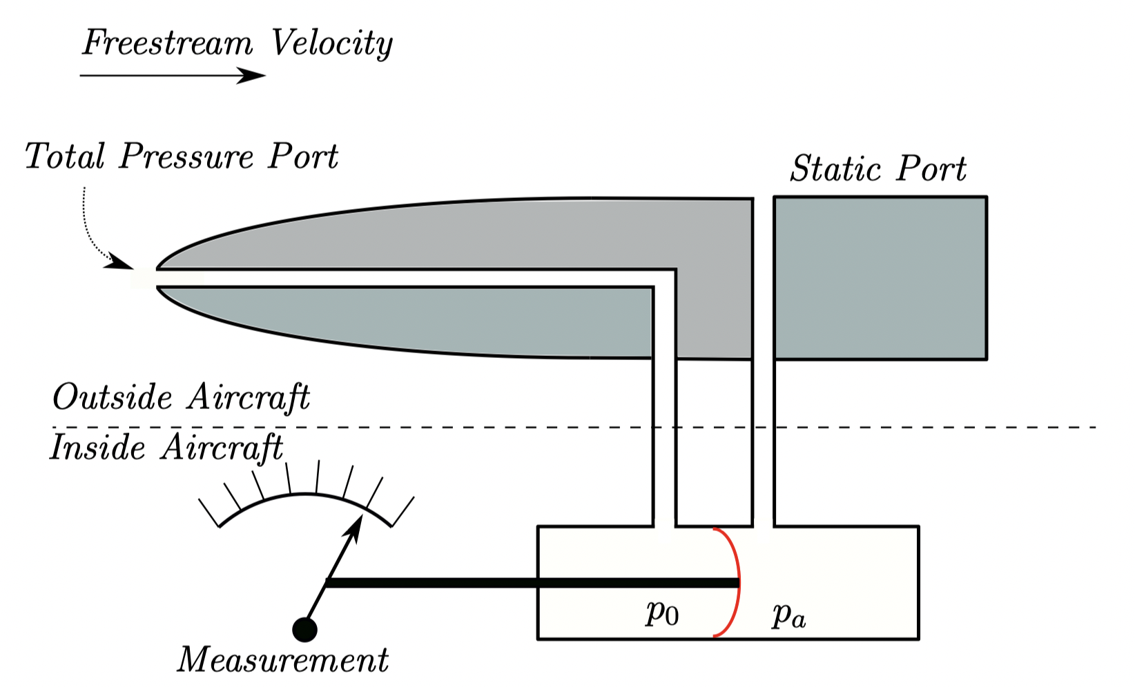
Aircraft Pitot-Static Measurement Device
Calibrated Airspeed
To avoid having to measure and , rather than using the pitot-static to measure , aircraft Engineers calibrated their devices to provide the correct value of true airspeed at sea-level ISA density and pressure. This provides us with calibrated airspeed, /CAS, which is only the same as true airspeed at sea-level ISA conditions. can be calculated via the following equation:
where we can see that the sea-level pressure has been replaced with the actual pressure. In practice, this correction is applied as a multiplier between CAS and EAS:
where
Since is only dependent on the the aircraft speed, and the the aircraft altitude, it can be calculated and tabulated - see the table below for the pressure correction factor:
| h, ft | Calibrated Airspeed, kn | |||||||||||||||||
|---|---|---|---|---|---|---|---|---|---|---|---|---|---|---|---|---|---|---|
| 100 | 125 | 150 | 175 | 200 | 225 | 250 | 275 | 300 | ||||||||||
| 5000 | 0.999 | 0.999 | 0.999 | 0.998 | 0.998 | 0.997 | 0.997 | 0.996 | 0.995 | |||||||||
| 10000 | 0.999 | 0.998 | 0.997 | 0.996 | 0.995 | 0.994 | 0.992 | 0.991 | 0.989 | |||||||||
| 15000 | 0.998 | 0.997 | 0.995 | 0.994 | 0.992 | 0.990 | 0.987 | 0.985 | 0.982 | |||||||||
| 20000 | 0.997 | 0.995 | 0.993 | 0.990 | 0.987 | 0.984 | 0.981 | 0.977 | 0.973 | |||||||||
| 25000 | 0.995 | 0.993 | 0.990 | 0.986 | 0.982 | 0.978 | 0.973 | 0.968 | 0.963 | |||||||||
| 30000 | 0.993 | 0.990 | 0.986 | 0.981 | 0.975 | 0.970 | 0.963 | 0.957 | 0.950 | |||||||||
| 35000 | 0.991 | 0.986 | 0.981 | 0.974 | 0.967 | 0.959 | 0.951 | 0.943 | 0.934 | |||||||||
| 40000 | 0.988 | 0.982 | 0.974 | 0.966 | 0.957 | 0.947 | 0.937 | 0.926 | 0.916 | |||||||||
| 45000 | 0.984 | 0.976 | 0.966 | 0.956 | 0.944 | 0.932 | 0.920 | 0.907 | 0.895 | |||||||||
| 50000 | 0.979 | 0.969 | 0.957 | 0.944 | 0.930 | 0.915 | 0.901 | 0.886 | 0.871 | |||||||||
Intermediate values are found via linear interpolation - you should be comfortable with doing this by hand, or by writing code. An example code is provided below that provides two-dimensional interpolation for any values - you can use this function to find out the pressure correction factor - use the syntax f_correction(VC, h) (both of these have default values, so you don’t need to provide either).
True Airspeed
Finally, True Airspeed may be calculated from Equivalent Airspeed, by accounting for the actual density at the correct altitude:
Where we may get the density at different altitudes from standard tables of the atmospheric properties. These are available in the original PDF notes. What we’ll use more regularly is either atmosisa in MATLAB or ambiance in Python.
If you can’t get the following to work - then you might need to install ambiance. Try pip install ambiance in your terminal window. See here for more instructions: https://pypi.org/project/ambiance/
Using ambiance to define the density, we can create a function, sigma_density (it’s a good idea to make function handles descriptive, and there tend to be lots of sigma functions that mean important things in programming languages). This function will return the density ratio for a given altitude provided in metres or feet - bearing in mind than the units for ambiance are metres.
A word about atmospheres
The ambiance module for Python implments the ICAO (International Civial Aviation Organisation) atmopshere, which is an extension of ISA (International Standard Atmosphere).
Printed in the old notes is the US Standard Atmosphere, which is another extension of the ISA model.
Both are equal in the ranges used in this course - but in the printed tables, the values have been truncated. This can lead to differences when interpolating from the table, and when using the routines. See the code dropdown below to understand this further.
The inputs can also be numpy arrays
Approximate density correction
For altitudes below about 16km, the approximation can be used
where is the altitude in .
The error in this approximation is easily shown using the functions created above:
Why use EAS?
Equivalent airspeed is actually very useful (though pilots tend not to actually use it, annoyingly). We tend to define as , which means that aerodynamic coefficients remain the same for a given and .
It is useful to see that the Equivalent Air Speed (EAS) for a given flight condition, , is the speed which if flown at standard sea level density () would give the same aerodynamic loads, for the same aerodynamic configuration, constant .
This is useful for simplicity of calculations, but is also useful for ease of flight - stall will always occur at the same angle, for the same EAS, regardless of flight altitude. Structural limits are always defined in EAS for the same reason, as the loads are constant at any altitude for the same EAS.
Summary of Corrections
We can remember the order of corrections by the mnemonic “ICE-T”, with the relative magnitudes of the velocities given by the shape that loosely looks like a square root -
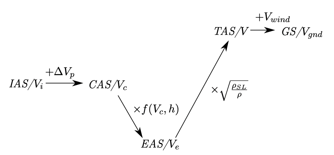
Airspeed Corrections
Problems:
Below are a range of numerical and theoretical questions. Some of the numerical questions have random numbers that change each time the notes get updated - so you’re not going crazy if you thought it was different last time.
Try and go through the questions on your own before looking at the solutions - questions you’ll face in tests/exams will be similar but not exactly the same, so you need to be able to understand the why of the solution rather than just following an algorithm.
Problem 1.1 - Conversion between airspeeds
An aircraft is flying at an altitude of 35000ft, with a calibrated airspeed of 195kn, with a 10kn headwind:
a) How long will it take to cover 100 miles?
b) How long will it take to cover 200km?
c) If instead of = 195kn, you have = 195kn, with a position error of , what do the above answers change to?
Try and tackle the problem yourself before you see the solution below. The numbers in this problem will change each time the notes are updated.
Click to show the solution...
The first step is to take Vc to Ve via the pressure correction.
For the altitude of 35000ft, with a calibrated airspeed of 195kn, the pressure correction can be interpolated from table using the function created earlier with syntax press_correction = f_correction(35000, 195).
This gives a value of 0.967 for the pressure correction, and this determination pf the equivalent airspeed from so, 192.489kn.
For EAS to TAS, the density ratio is required - , and this is found to be 0.311kn. Since this is an altitude above sea level, this has to be a number smaller than one - if it’s not, then you’ve done something wrong.
True airspeed is obtained from the relationship which yields =345.399kn.
Note that at no point have the units had to be converted into SI to make the corrections - that’s the smart part of the density and pressure corrections; they are both non-dimensional corrections. If you have velocity in knots, you use them and get velocity in knots out.
Since the wind is a headwind, this is subtracted from the value above to yield the groundspeed in knots as 335.399kn. This gives the speed of the aircraft relative to the ground, and hence the speed we require for distance/time calculations.
With the velocity in knots it may be easily converted to m/s by multiplying by 0.5144444 which yields =172.544m/s.
100 miles is 160,934m, and hence this is covered in 932.7s or 15 minutes, 32 seconds
200 km is 200,000, and hence this is covered in 1159.1s or 19 minutes, 19 seconds
For the last part of the question, this is solved by recalling that and hence the speeds calculated are now:
= 201.000kn
= 194.303kn
= 348.654kn
= 358.654kn = 184.508m/s
The times taken are found to be 14 minutes, 32 seconds and 18 minutes, 3 seconds, for a respective 1 minutes, 0 seconds and 1 minutes, 15 seconds faster.
Problem 1.2 - Theory
a) When converting between different airspeeds, how can you ‘sense check’ your numbers?
Click to show the solution...
Look at the square-root symbol for ICE-T Defining Aircraft ‘Speed’. This shows the respective magnitude of the velocities you should expect to find.
Once you have the true airspeed, you should also compare it to the type of aircraft listed (if one is). The speed of sound is about 340m/s at sea-level - so if you’ve been given a light commuter aircraft, and you’ve found a true airspeed of 500m/s then something is wrong. (You probably got the knots to metre/s conversion wrong - see here
b) What is the significance of “equivalent airspeed”, and why is it preferable to use when defining limiting speeds for aircraft
Click to show the solution...
For a given angle of attack, the dimensional lift on a given aircraft will be the same for constant at any altitude. This is not the same for any of the other airspeeds.
Hence - the stall speed (which we will calculate soon) is constant with altitude when defined in EAS, as is the “never exceed” speed (provided has been defined due to aerodymamic structural limitations.
c) In what cases could you find that your true airspeed is less than your calibrated airspeed?
Click to show the solution...
Flight below sea-level, or if you’ve made a mistake.
d) For what conditions is EAS equivalent to TAS?
Click to show the solution...
Flight at sea-level.