Flight Dynamicsdraft
Dynamic Stability
In this course, the equations of motion have been developed in a Newtonian framework - these, in conjunction with the relationship between body rates and the time rate of change of the Euler angles, allow us to describe full unconstrained flight of a six degree of freedom aircraft.
Regarding static stability, some basic static stability properties of fixed-wing aircraft were explored - what the immediate tendency of the aircraft is following a disturbance from trim. In the previous module we developed the equations of motion into two sets of uncoupled linearised equations of motion, representing the longitudinal and lateral/directional motions of fixed wing aircraft.
In this final module, we look at the dynamic stability characteristics of an aircraft - how the aircraft actually responds with time, and how the response to basic pilot inputs may be determined. The stability of any dynamic system is governed by consideration of its free (unforced) motion. Its response to an input (an aircraft control) is determined by the response of the system to forcing.
A simple example that helps us understand dynamic systems is the mass/spring/damper system as shown:
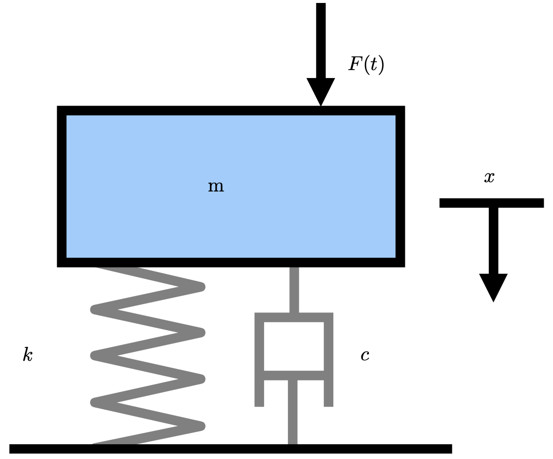
Mass Spring Damper System
This system is governed by the equation of motion:
where is the displacement, is the mass, is the damping, is the spring stiffness, and is the input forcing. For free motion, :
which we can represent as:
where is the undamped natural frequency of the system ( for this case) and is the damping ratio of the system ( for this case).
The stability of this system is given by solution of Eq (1) directly. The general solution is found by assuming that the solution will have the form , hence . Substitution of this into Equation (1) yields the characteristic equation:
the roots of which are
by superposition, the general solution is
where
Because , the radicand may be positive, negative, or zero. These three possibilities give rise to three different types of damped motion, and the difference in behaviour may be classified according to the table below
| Type of Motion | Motion Characteristics | ||
|---|---|---|---|
| ’Overdamped’ | Real, negative, distinct | Motion decays to zero over a period of time, , with zero oscillation. | |
| ‘Critically Damped’ | Real, negative, equal | Motion decays to zero over a period of time , where is the shortest possible time to return to equilibrium for this system. | |
| ‘Underdamped’ | Complex | Motion returns toward, and beyond zero in time where is smaller than the time for the critically damped case. Motion will overshoot and exhibit harmonic oscillation. |
different values of are demonstrated for free vibration of the mass-spring-damper system, with the maxima/minima of the underdamped cases shown, to show the change in the damped natural frequencies of the system. Furthermore, the period of the oscillatory systems are used to show the damped natural frequency which is then compared with the value from the formula. Hopefully this should elucidate the difference between the two sorts of natural frequencies.
Most aircraft problems that we will look at exhibit underdamped motion and Eq (4)1 can be re-written as:
we introduce a parameter , which represents the \textsl{damped natural frequency}, which allows us to express this as
Where and . Inspection of (5) shows an oscillation with angular frequency , and a decaying amplitude with time. This is demonstrated below:
To determine the system’s forced response to an input, we set to a given value, and solve. We will explore this via examples for real aircraft.
Determining Stability - Eigenvalues
We have already shown the characteristic equation of the mass spring damper system to be:
Note that if we had taken the Laplace Transform of the equation of motion with zero initial conditions, we would have arrived at the characteristic equation in terms of the Laplace Operator,
Clearly equations (2) and (6) are equivalent, hence the poles and eigenvalues are equivalent. Since we know that the poles of the system give information on its stability, then we can further surmise that its eigenvalues do the same. Furthermore, we have shown that the eigenvalues are given by the solution of the characteristic equation:
hence we can see that the system’s eigenvalues and therefor its stability is a function of both the natural frequency and the damping.
For mechanical systems, damping can only be positive, and hence the term will always be positive. This is a consequence of physical damping being a removal of kinetic energy - hence this always causes oscillations to decrease in amplitude. For aircraft, however, the interplay of aerodynamic and propulsive forcing causing a conversion between potential and kinetic energy can give rise to negative damping, whereby energy is added to a system. This causes oscillations which increase with time. For solution of the aircraft equations of motion, the eigenvalues may be real or complex, and have a positive or negative real component. This gives rise to four possibilities as shown in the table below:
| Dynamic Response | |
|---|---|
| Real and Negative | This denotes an exponential decay or a convergence. This is indicative of static stability. |
| Real and Positive | This denotes an exponential increase or a divergence. This is indicative of static instability. |
| Complex, | This denotes an oscillatory motion with a decreasing amplitude. This is indicative of dynamic stability. |
| Complex, | This denotes an oscillatory motion with an increasing amplitude. This is indicative of dynamic instability. |
you will see from the above that the existence of a complex root gives rise to dynamic behaviour, and its sign does not matter.
Period and time to half amplitude
If we consider the general eigenvalue and decompose into its imaginary and real parts:
Which gives the response
For the oscillatory modes, the angular frequency is given by the imaginary part of the eigenvalue - hence the period of any oscillations, , is given by
with a frequency given by
The decay rate of the oscillatory behaviour is given by the real part of the eigenvalue - hence this determines the damping. When looking at aircraft modes of motion, we tend to talk about the ‘time to half amplitude’ for convergent modes, or the ‘time to double amplitude’ for a divergent mode. Since the amplitude of the oscillation is given:
hence for a stable system, the time to half amplitude, , is given by:
Note that as the time to half amplitude is only calculated for a stable system where the eigenvalue will be negative, the time will be a positive value. Similarly for an unstable system, the time to double amplitude is found from
Again, since the time to double amplitude is only calculated for an unstable system where the eigenvalue will be positive, the time will always be a positive value.
Note that as presented above, we are assuming the dimensional equations of motion. If we are using them in their nondimensional form, then the reduced time is calculated and the answers must be multiplied by .
Damped and Undamped Natural Frequencies
The damped natural frequency, , is the frequency at which the actual system will exhibit oscillatory behaviour if measured in the real world, subject to damping. The natural frequency, , of the system is a frequency that the system would vibrate if the oscillatory behaviour were influenced by the system stiffness alone.
In short, we can get the two from:
but it’s not always apparent why this is the case. We know that a second order system will have the general form of:
and we have further shown that the eigenvalues found determine the modal characteristics of the system. Since these are the roots of the characteristic equation we can write the above as:
the right hand side can be mutlipled out to give
which, given the relationship between damped and undamped natural frequncies as
may be readily rearranged to give the two expressions for natural frequency.
The stability of a multiple degree of freedom system
The theory presented above has been developed in a theory that is easily extensible to multiple degree of freedom systems. The general first order ODE can be represented as
This equation represents a system of equations where is the number of states and degrees of freedom. Hence for the preceding analysis, , whereas it will be for our aircraft problem. The general solution will be2:
in vector form
similarly, differentiating and substituting into Eq. (7)
which is an eigenvalue (matrix/vector) problem and hence we can write
The trivial solution is zero displacement, , but more useful solution is given by the determinant
Equation (9) is the characteristic equation of a multiple degree of freedom system, and will be a polynomial of order , yielding eigenvalues dictating the system stability. If any single value is unstable, then the aircraft is deemed dynamically unstable. Similarly, if any of the eigenvalues give a complex pair, then the characteristic motion will be oscillatory as the equations are coupled.
Once the eigenvalues have been solved, each of these may be substituted into Eq. (8) to solve for the vector of amplitudes to give vectors of amplitudes. The magnitudes of each respect state motion help us to determine which variables correspond to which eigenvalue (or which eigenvalues correspond to which mode of the aircraft).
Before we can utilise the eigenvalues to tell us information about the modes of the aircraft, we will require an understanding of what each of the aircraft modes of motion comprises. The following section will describe what each mode is, in a physical sense before we delve into the governing mathematics.