Aircraft Equations of Motiondraft

Axes Transformations

The orientation of the body axis set within the Earth axis set is dictated by the aircraft’s attitude, defined by three angles, known as the Euler Angles:

Euler Angles

Yaw $(\psi)$ - The angle between the projection of $x_b$ on the plane of the earth, and the $x$ axis, defined as rotation around $z$ .
Pitch $(\theta)$ - The angle between the aircraft $x_b$ axis, and the earth $x_e/y_e$ plane, defined as rotation around intermediate axis $y_1$ .
Roll $(\phi)$ - The angle between the aircraft $x_b/y_b$ plane, and the intermediate $x_2/y_2$ plane - defined as rotation around $x_2$ .

A transformation matrix is desired to enable the definition of, for two axes systems with co-located origins, what a set of co-ordinates in one axes system is in the other. That is, at this stage we are not concerned with axial translation and we only wish to look at the effect of angular translation (yaw, pitch, and roll).

\begin{bmatrix}X_b\\Y_b\\Z_b\end{bmatrix}= \left[T(\psi, \theta, \phi)\right]\begin{bmatrix}X_e\\Y_e\\Z_e\end{bmatrix}

We define $[T]$ by performing a three individual rotations, involving two intermediate axes systems, and combining the result.

Earth axes to intermediate axes $[x_1, y_1, z_1]$ through Yaw, $\psi$

We perform an Euler transform to define $x_E,y_E$ in the intermediate axes $x_1,y_1$ , noting that $z_e=z_1$ . You may have seen Euler transforms before, but they can be confusing, and are not clearly described in many textbooks - and, occasionally, taught incorrectly. Euler transforms don’t just appear in Flight Mechanics - if you do anything with rotation, then they come in handy all the time - so mastering this will put you in excellent stead for rotary aerodynamics.

The key to getting an Euler transform correct is to understand what you’re doing - you are trying to describe a point that has original co-ordinates $x_e, y_e$ in the earth axis system, and wish wish to determine what co-ordinates it would have in this new axis system $x_1, y_1$ . We can use basic trigonometry to work this out. Apply the following rules, and you should be okay:

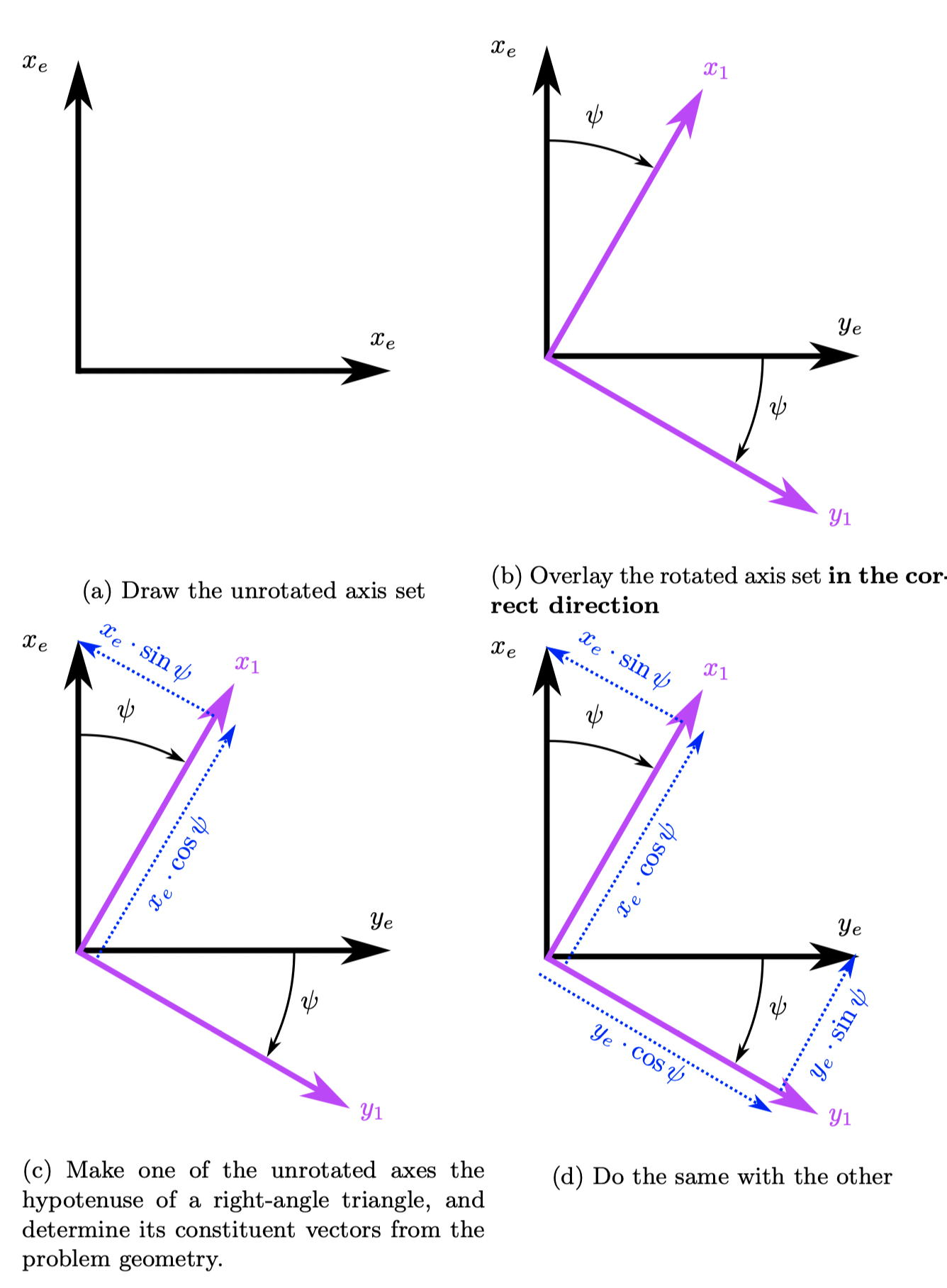
Draw your unrotated axis set in any arbitrary orientation. Figure Fig. 1 (a).
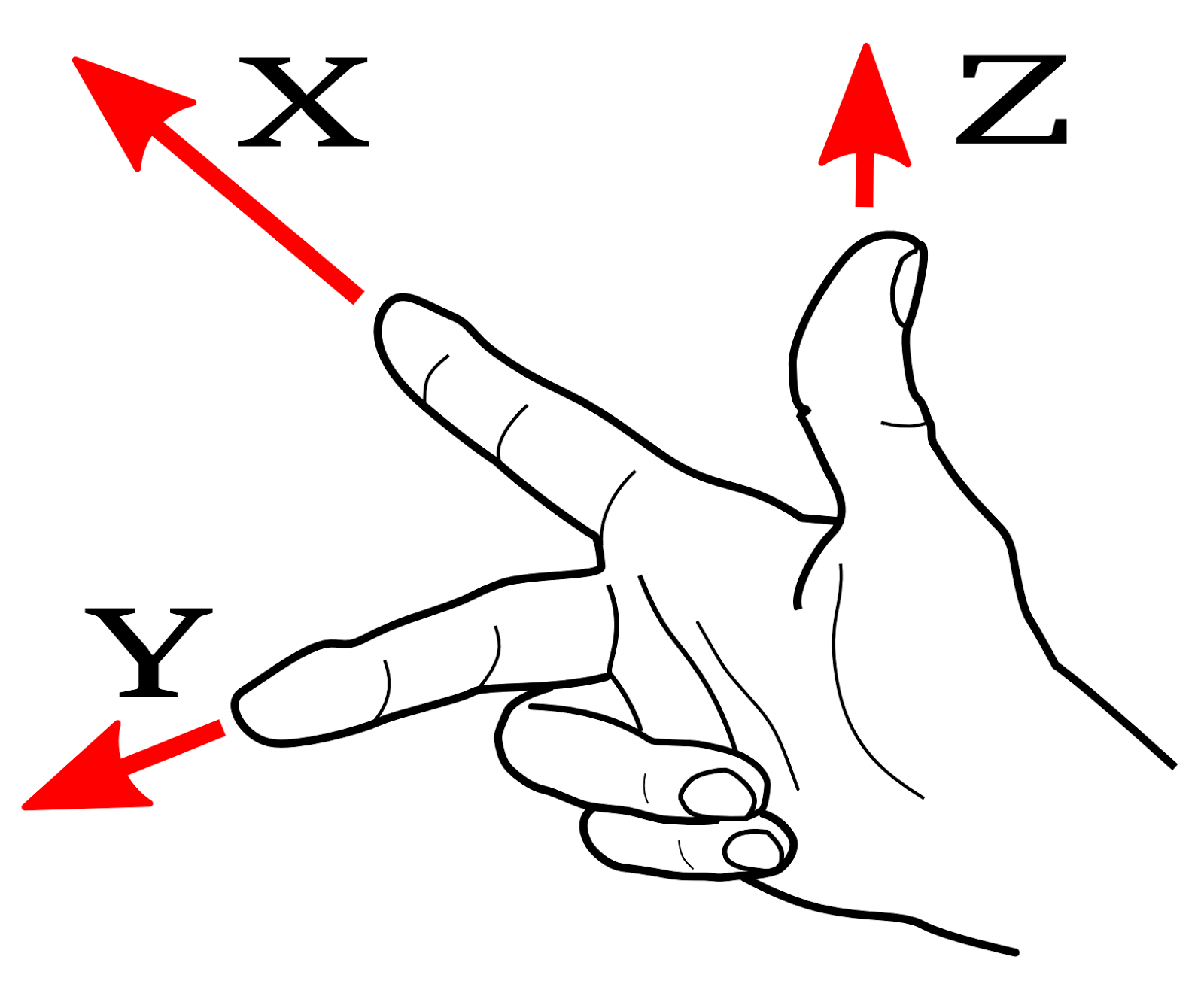
Use your right hand to orient the axis system (see Figure Fig. 2), and determine the direction of the positive third axis (in or out of the page). In Figure Fig. 1 (a), the $z$ -axis is positive into the page.
The right hand screw rule - See Figure Fig. 3 - defines the direction of positive rotation - for Figure, this is a clockwise rotation. Draw your rotated axes set at some arbitrary positive angle of rotation - in this case, through Yaw ( $\psi$ ) - Figure Fig. 1 (b) .
Recall that you are defining what the point $x_e,y_e$ would be in this new axis set - we can do this for each of them individually. Pick one, say $x_e$ , and draw a right-angle triangle with the unrotated axis ( $x_e$ ) as the hypotenuse. The adjacent side defines the component of $x_e$ along $x_1$ , whilst the opposite side defines the component of $x_e$ along $y_1$ which we can see is negative in this case - Figure Fig. 1 (c).
Do the same for the remaining unrotated axis - Figure Fig. 1 (d).
Collect the components are along the rotated X-axis, $x_1$ : $x_1=x_e\cdot\cos\psi+y_e\cdot\sin\psi$
Collect the components are along the rotated Y-axis, $y_1$ : $y_1=y_e\cdot\cos\psi-x_e\cdot\sin\psi$ noting the minus sign in this one, as $x_e\cdot\sin\psi$ was pointed in the negative $y_e$ direction.
We have already stated that $z_1=z_e$ , so we can write the above in matrix form:

\begin{aligned} \vec{R_1}&=\left[T_1\right]\vec{ R_e}\\ \begin{bmatrix}x_1\\y_1\\z_1\end{bmatrix}&=\begin{bmatrix}\cos\psi & \sin\psi & 0\\-\sin\psi & \cos\psi & 0\\ 0 & 0 & 1\end{bmatrix}\begin{bmatrix}x_e\\y_e\\z_e\end{bmatrix} \end{aligned}

Check that you have a matrix with; four trig terms, four zeros, and a single unity term (1). The top-left and bottom-right trig term will be a positive cosine. The top-right, and bottom-left trig term will be a sine - one positive, one negative. The (1) will be in a row and column of its own, and everything else will be zero. If your transformation matrix doesn’t follow these rules, you’ve messed up.

Fig. 1:
Step to create the Euler matrix from $O_{e}$ to $O$ (Earth to body)

Fig. 2:
The rule for assigning a correct right-handed Cartesian axis system

Fig. 3:
The rule for assigning a correct right-handed rotation direction

Intermediate Axes 1 to Intermediate Axes 2 through Pitch, $\theta$

So far we have only yawed our axis system, we need to pitch it next. We do exactly the same as before. Figure Fig. 4 shows the aecond rotation through pitch, $\theta$ .

To determine the second transformation matrix:

\begin{aligned} \begin{bmatrix}x_2\\y_2\\z_2\end{bmatrix}&=\begin{bmatrix}\cos\theta & 0 & -\sin\theta\\ 0 & 1 & 0 \\ \sin\theta & 0 & \cos\theta\end{bmatrix}\begin{bmatrix}x_1\\y_1\\z_1\end{bmatrix}\\ \vec{R_2}&=[T_2]\vec{R_1}\\ &=[T_2][T_1]\vec{R_e}\end{aligned}

Fig. 4: Euler Rotation from Intermediate Axes 1 to Intermediate Axes 2 through Pitch,

\theta

Intermediate Axes 2 to Body Axes through Roll, $\phi$

Figure Fig. 5 shows the final rotation through roll, $\phi$ .

\begin{aligned} \begin{bmatrix}x\\y\\z\end{bmatrix}&=\begin{bmatrix}1 & 0 & 0\\0 & \cos\phi & \sin\phi \\ 0 & -\sin\phi & \cos\phi \end{bmatrix}\begin{bmatrix}x_2\\y_2\\z_2\end{bmatrix}\\ \vec{R}&=[T_3]\vec{R_2}\\ &=[T_3][T_2][T_1]\vec{R_e}\end{aligned}

Fig. 5: Euler Rotation from Intermediate Axes 2 to Body Axes through Roll,

\phi

Total Transformation Matrix

Since we have now defined $[T_1]$ , $[T_2]$ , and $[T_3]$ , we can perform the matrix multiplication and express $[T]$ .

\begin{aligned} &=[T_3][T_2][T_1]\\ &=\begin{bmatrix}1 & 0 & 0\\0 & \cos\phi & \sin\phi \\ 0 & -\sin\phi & \cos\phi \end{bmatrix}\begin{bmatrix}\cos\theta & 0 & -\sin\theta\\ 0 & 1 & 0 \\ \sin\theta & 0 & \cos\theta\end{bmatrix}\begin{bmatrix}\cos\psi & \sin\psi & 0\\-\sin\psi & \cos\psi & 0\\ 0 & 0 & 1\end{bmatrix}\\ &= \begin{bmatrix}\cos\theta\cos\psi & \cos\theta\sin\psi & -\sin\theta \\ -\cos\phi\sin\psi + \sin\phi\sin\theta\cos\psi & \cos\phi\cos\psi + \sin\phi\sin\theta\sin\psi & \sin\phi\cos\theta \\ \sin\phi\sin\psi + \cos\phi\sin\theta\cos\psi & -\sin\phi\cos\psi + \cos\phi\sin\theta\sin\psi & \cos\phi\cos\theta\end{bmatrix}\end{aligned}

Now we can convert between Earth axes and body axes and vice versa:

\begin{aligned} \vec{R} &= [T]\vec{R_e}\\ \vec{R_e} &= [T]^{-1}\vec{R}\end{aligned}

Handily, $[T]$ is orthogonal, meaning $[T][T]^T=[I]$ , thus $[T]^{-1}=[T]^T$ . Hence:

[T]^{-1}= \begin{bmatrix}\cos\theta\cos\psi & \cos\theta\sin\psi & -\sin\theta \\ -\cos\phi\sin\psi + \sin\phi\sin\theta\cos\psi & \cos\phi\cos\psi + \sin\phi\sin\theta\sin\psi & \sin\phi\cos\theta \\ \sin\phi\sin\psi + \cos\phi\sin\theta\cos\psi & -\sin\phi\cos\psi + \cos\phi\sin\theta\sin\psi & \cos\phi\cos\theta\end{bmatrix}

Usage

It is easiest to define the gravitational forces in Earth axes, as has already been shown in Equation (1):

\vec{F}_{G_E} = \begin{bmatrix}0\\0\\W\end{bmatrix}_{e} =\begin{bmatrix}0\\0\\ mg\end{bmatrix}_{e}

For development of the aircraft equations of motion, it is desired to express all forces in body axes, so we write:

\begin{aligned} \vec{F}_{G_b} &= \left[T\right]\vec{F}_{G_e}\\ &= \begin{bmatrix}\cos\theta\cos\psi & \cos\theta\sin\psi & -\sin\theta \\ -\cos\phi\sin\psi + \sin\phi\sin\theta\cos\psi & \cos\phi\cos\psi + \sin\phi\sin\theta\sin\psi & \sin\phi\cos\theta \\ \sin\phi\sin\psi + \cos\phi\sin\theta\cos\psi & -\sin\phi\cos\psi + \cos\phi\sin\theta\sin\psi & \cos\phi\cos\theta\end{bmatrix}\begin{bmatrix}0\\0\\mg\end{bmatrix} \end{aligned}

= \begin{bmatrix}-mg\cdot\sin\theta\\mg\cdot \sin\phi\cos\theta\\mg\cdot \cos\phi\cos\theta\end{bmatrix}\tag{1}

From Stability Axes to Body Axes

The transformation from Stability Axes to Body axes is another Euler transform, which you should be capable of doing now. Note that the definition of $\alpha$ is such that for a positive angle of attack, $V_f$ approaches the aircraft from underneath, thus providing a $w$ component. It may be shown that:

\begin{aligned} \begin{bmatrix}x_b\\y_b\\z_b\end{bmatrix} &= \begin{bmatrix}\cos\alpha & 0 & -\sin\alpha\\0 & 1 & 0\\\sin\alpha & 0 & \cos\alpha\end{bmatrix}\begin{bmatrix}x_w\\y_w\\z_w\end{bmatrix}\end{aligned}\tag{2}

Usage

This transformation is used to convert the aerodynamic force vector into body axes:

\begin{aligned} \begin{bmatrix}F_{A_x}\\F_{A_y}\\F_{A_z}\end{bmatrix}_b &= \begin{bmatrix}\cos\alpha & 0 & -\sin\alpha\\0 & 1 & 0\\\sin\alpha & 0 & \cos\alpha\end{bmatrix}\begin{bmatrix}F_{A_x}\\F_{A_y}\\F_{A_z}\end{bmatrix}_s\nonumber\\ &= \begin{bmatrix}\cos\alpha & 0 & -\sin\alpha\\0 & 1 & 0\\\sin\alpha & 0 & \cos\alpha\end{bmatrix}\begin{bmatrix}-D\\F_{A_y}\\-L\end{bmatrix}_s\nonumber\end{aligned}

=\begin{bmatrix}-D\cos\alpha + L\sin\alpha\\ F_{A_y}\\ -D\sin\alpha - L\cos\alpha\end{bmatrix}\tag{3}

a sense check of the forces in Equation (3) may be performed - the body axial force has a large component aftward because of drag, and a small component acting forward (in body axes) due to lift. Lift acts ‘upward’ for positive AoA, as would be expected.

Fig. 6: Aerodynamic Angles

Euler Rates

It is important to understand that the Euler angles are not defined in the same axis set (yaw is defined in earth axes, pitch is defined in intermediate axes 1, and roll is defined in intermediate exes 2).

Consequently:

\begin{bmatrix} P\\Q\\ R \end{bmatrix}\neq\left[T\right] \begin{bmatrix} \dot{\phi}\\\dot{\theta}\\\dot{\psi}\end{bmatrix}

A rate gyro in the aircraft with principal axes aligned with the aircraft axes will measure $\left[P, Q, R\right]$ which are, by definition, the body angular rates. Since we define the relationship between body axes and earth axes by the Euler angles, we require the means to translate between body rates and Euler rates. We construct a transformation matrix based on the sequence of rotations, whereby each Euler angle rate has components in body $[x,y,z]$ :

First: Angular velocity about Earth axes, yaw ( $z_e,\dot{\psi}$ ):

\begin{aligned} \begin{bmatrix} \dot{\psi}_x\\ \dot{\psi}_y\\ \dot{\psi}_z \end{bmatrix}_b &= [T_3]\cdot[T_2]\cdot[T_1]\cdot \begin{bmatrix} 0\\ 0\\ \dot{\psi} \end{bmatrix}\nonumber\\ &= \begin{bmatrix} -\dot{\psi}\sin\theta\\ \dot{\psi}\sin\psi\cos\theta\\ \dot{\psi}\cos\psi\cos\theta \end{bmatrix}\end{aligned}

Second: Angular velocity about intermediate axes one, pitch ( $y_1,\dot{\theta}$ ):

\begin{aligned} \begin{bmatrix} \dot{\theta}_x\\ \dot{\theta}_y\\ \dot{\theta}_z \end{bmatrix}_b &= [T_3]\cdot[T_2]\cdot \begin{bmatrix} 0\\ \dot{\theta}\\ 0 \end{bmatrix}\nonumber\\ &= \begin{bmatrix} 0\\ \dot{\theta}\cos\phi\\ -\dot{\theta}\sin\phi \end{bmatrix}\end{aligned}

Third: Angular velocity about intermediate axes two, roll ( $x_2,\dot{\phi}$ ):

\begin{aligned} \begin{bmatrix} \dot{\phi}_x\\ \dot{\phi}_y\\ \dot{\phi}_z \end{bmatrix}_b &= [T_3]\cdot \begin{bmatrix} \dot{\phi}\\ 0\\ 0 \end{bmatrix}\nonumber\\ &= \begin{bmatrix} \dot{\phi}\\ 0\\ 0 \end{bmatrix}\end{aligned}

So the body angular rate vector is equal to the total rate of change in each axis because of the three Euler rates, or

\begin{aligned} \vec{\omega } &= \dot{\vec{\phi}} + \dot{\vec{\theta}} + \dot{\vec{\psi}}\nonumber\\ &= \begin{bmatrix} \dot{\phi}\\ 0\\ 0 \end{bmatrix} + \begin{bmatrix} 0\\ \dot{\theta}\cos\phi\\ -\dot{\theta}\sin\phi \end{bmatrix} + \begin{bmatrix} \dot{\psi}\sin\theta\\ \dot{\psi}\sin\psi\cos\theta\\ \dot{\psi}\cos\psi\cos\theta \end{bmatrix}\nonumber\\ &= \begin{bmatrix} 1 & 0 & -\sin\theta\\ 0 & \cos\phi & \sin\phi\cos\theta\\ 0 & -\sin\phi & \cos\phi\cos\theta \end{bmatrix}\begin{bmatrix} \dot{\phi}\\\dot{\theta}\\\dot{\psi}\end{bmatrix} \end{aligned}

The matrix above is not orthogonal, but if we use the inverse of the three Euler matrices, we can construct the inverse of the matrix above (or invert the 3 x 3 manually)

\begin{aligned} \begin{bmatrix} \dot{\phi}\\\dot{\theta}\\\dot{\psi}\end{bmatrix} &= \begin{bmatrix} 1 & \sin\phi\tan\theta & \cos\phi\tan\theta\\ 0 & \cos\phi & -\sin\phi \\ 0 & \frac{\sin\phi}{\cos\theta} & \frac{\cos\phi}{\cos\theta} \end{bmatrix}\begin{bmatrix} P\\Q\\R\end{bmatrix}\end{aligned}\tag{4}

It should be apparent that for the case of $\theta=90^\circ$ , the matrix above becomes singular, and hence for pitch vertically upwards, a relationship between body and Euler rates cannot be defined. This is known as ‘gimbal lock’ - but fortunately, for our purposes, we shall not be dealing with aircraft flying straight upward!

Whilst aerodynamic forces are generally defined in stability axes, the aircraft velocity vector is defined in wind axes - hence we need to be able to relate the incident flow to Earth and body axes, respectively.
We relate $\vec{V}_f$ to $[U, V, W]$ via the aerodynamic angles¹.

Trajectory Angles

The trajectory angles define the orientation of the velocity vector $\vec{V}_f$ in earth axes. The angles are:

Track angle, $\tau$
Flight path angle, $\gamma$

Which we define as the aircraft velocity resolved into earth axis components:

\begin{aligned} \begin{split} U_e &= V_f\cdot\cos\gamma\cdot\cos\tau\\ V_e &= V_f\cdot\cos\gamma\cdot\sin\tau\\ W_e &= V_f\cdot\sin\gamma \end{split}\end{aligned}\tag{5}

The flight path angle is the angle between the velocity vector and its projection in the $x_e, y_e$ plane. The track angle is the angle between that projection and due north, $x_e$ .

Caution must be taken as these angles are defined in the opposite order to aerodynamic angles. That is, $\vec{V}_f^\prime$ is the projection of $\vec{V}_f$ in the $x_e,y_e$ plane. Hence $\vec{V}_f^\prime\triangleq\vec{V}_f\cos\gamma$ .

The remainder of Eq. (5) should follow from basic trigonometry.

Fig. 7: Trajectory Angles

Reference Angles on the same planes:

We can overlay the flight path $\gamma$ and angle of attack $\alpha$ on the same diagram (for the case of zero sideslip, track) - Figure Fig. 8.

We can do the same for the track angle $\tau$ and the aircraft sideslip angle $\beta$ - Figure Fig. 9.

Fig. 8: Reference angles on ZX plane

Fig. 9: Reference angles on XY plane

Numerial Example

Aircraft accident investigators wish to calculate the descent rate of an aircraft at the moment of impact into the ocean. The flight data recorder outputs are in terms of the following aircraft variables:

Sideslip, yaw, pitch angles = 0

Roll angle = 60 $^\circ$

Angle of Attack = 30 $^\circ$

Airspeed = 120kn EAS

Click to see solution

We can calculate that 120kn = 61.728. From here we must calculate the body axes components:

\begin{aligned} U&= V_f\cdot\cos\alpha\cos\beta = 61.728\cdot\cos 30 = 53.485\text{m/s EAS}\\ V &=V_f\cdot\sin 0 = 0\\ W &=V_f\cdot\sin30\cos0 =30.864\text{m/s EAS} \end{aligned}

and we can convert to earth axes through the inverse Euler transformation matrix:

\begin{aligned} \vec{V}_e &= \left[T\right]^{-1}\vec{V}\\ &= \begin{bmatrix}\cos\theta\cos\psi & -\cos\phi\sin\psi + \sin\phi\sin\theta\cos\psi & \sin\phi\sin\psi + \cos\phi\sin\theta\cos\psi \\ \cos\phi\sin\psi & \cos\phi\cos\psi + \sin\phi\sin\theta\sin\psi & -\sin\phi\cos\psi + \cos\phi\sin\theta\sin\psi \\ -\sin\theta & \sin\phi\cos\theta & \cos\phi\cos\theta\end{bmatrix}\vec{V}\end{aligned}

Descent rate is simply $W_e$ , hence:

\begin{aligned} W_e &= 53.458\cdot\sin0 + 0\sin60\cdot\cos0 + 30.864\cos60\cos0\\ &= 15.432\text{m/s EAS}\end{aligned}

noting that $\vec{V}$ without a subscript is the velocity in body axes by definition ↩

Axes Transformations

Euler Angles

Earth axes to intermediate axes [x1,y1,z1][x_1, y_1, z_1][x1​,y1​,z1​] through Yaw, ψ\psiψ

Intermediate Axes 1 to Intermediate Axes 2 through Pitch, θ\thetaθ

Intermediate Axes 2 to Body Axes through Roll, ϕ\phiϕ

Total Transformation Matrix

Usage

From Stability Axes to Body Axes

Usage

Euler Rates

Velocity related to Earth and Body Axes

Trajectory Angles

Reference Angles on the same planes:

Numerial Example

Footnotes

Earth axes to intermediate axes $[x_1, y_1, z_1]$ through Yaw, $\psi$

Intermediate Axes 1 to Intermediate Axes 2 through Pitch, $\theta$

Intermediate Axes 2 to Body Axes through Roll, $\phi$