Linearisationdraft

The following is a direct adaptation of an example given in my own undergraduate notes - reproduced with permission. Thanks, Dougie.

Comparison of the Linear and Nonlinear Equations of Motion: Aircraft Simulation

The nonlinear equations of motion have been derived and will be repeated here:

m\begin{bmatrix} \dot{U} + QW - UR \\ \dot{V} + RU-PW\\\dot{W}+PV-QU\end{bmatrix}=\begin{matrix} -mg\sin\Theta - D\cos\alpha + L\sin\alpha + T\cos\Theta_T\\mg\sin\Phi\cos\Theta + F_{A_Y} + F_{T_Y}\\mg\cos\Phi\cos\Theta - D\sin\alpha - L\cos\alpha - T\sin\Theta_T\end{matrix}

\left[{\begin{matrix} \dot{P}\cdot I_{xx} \\ \dot{Q}\cdot I_{yy} \\\dot{R}\cdot I_{zz}\end{matrix}} \hspace{.5cm} \begin{matrix} + \\+\\+\end{matrix} \hspace{.5cm} {\begin{matrix} Q\cdot r\left(I_{zz} - I_{yy}\right) \\ P\cdot R\left(I_{xx} - I_{yy}\right) \\ P\cdot Q\left(I_{yy} - I_{xx}\right)\end{matrix}} \hspace{.5cm} \begin{matrix} - \\+\\+\end{matrix} \hspace{.5cm} {\begin{matrix}\left(\dot{R} + P\cdot Q\right) I_{xz} \\ \left(P^2 - R^2\right) I_{xz} \\ \left(Q\cdot R - \dot{P}\right) I_{xz}\end{matrix}} \right] = \begin{bmatrix} L \\ M \\ N\end{bmatrix}

\begin{aligned} \begin{bmatrix} P\\Q\\R\end{bmatrix} &= \begin{bmatrix} 1 & 0 & -\sin\Theta\\ 0 & \cos\Phi & \sin\Phi\cos\Theta\\ 0 & -\sin\Phi & \cos\Phi\cos\Theta \end{bmatrix}\begin{bmatrix} \dot{\Phi}\\\dot{\Theta}\\\dot{\Psi}\end{bmatrix}\end{aligned}

\begin{aligned} \begin{bmatrix} \dot{\Phi}\\\dot{\Theta}\\\dot{\Psi}\end{bmatrix}&= \begin{bmatrix} 1 & \sin\Phi\tan\Theta & \cos\Phi\tan\Theta\\ 0 & \cos\Phi & -\sin\Phi \\ 0 & \frac{\sin\Phi}{\cos\Theta} & \frac{\cos\Phi}{\cos\Theta} \end{bmatrix}\begin{bmatrix} P\\Q\\R\end{bmatrix}\end{aligned}

a simulation of this aircraft in the longitudinal plane will be presented in this section. By constraining to longitudinal motion only, the solution of the nonlinear equations is heavily simplified, but the analysis can be expanded for the unconstrained case and if we assume the thrust inclination is zero. The simplifying assumption is:

V=P=R=\Phi=\Psi=\Theta_0 = 0

and the equations describing longitudinal flight may now be we written:

\begin{aligned} m\left(\dot{U} + Q\,W\right) &= T - D\cos\alpha + L\cos\alpha - mg\,\sin\Theta\\ m\left(\dot{W} - Q\,U\right) &= -L\cos\alpha - D\sin\alpha+ mg\,\cos\Theta\\ I_{yy}\,\dot{Q} &= M_A - T\,\Delta_{zT}\\ \dot{\Theta}&=Q\end{aligned}

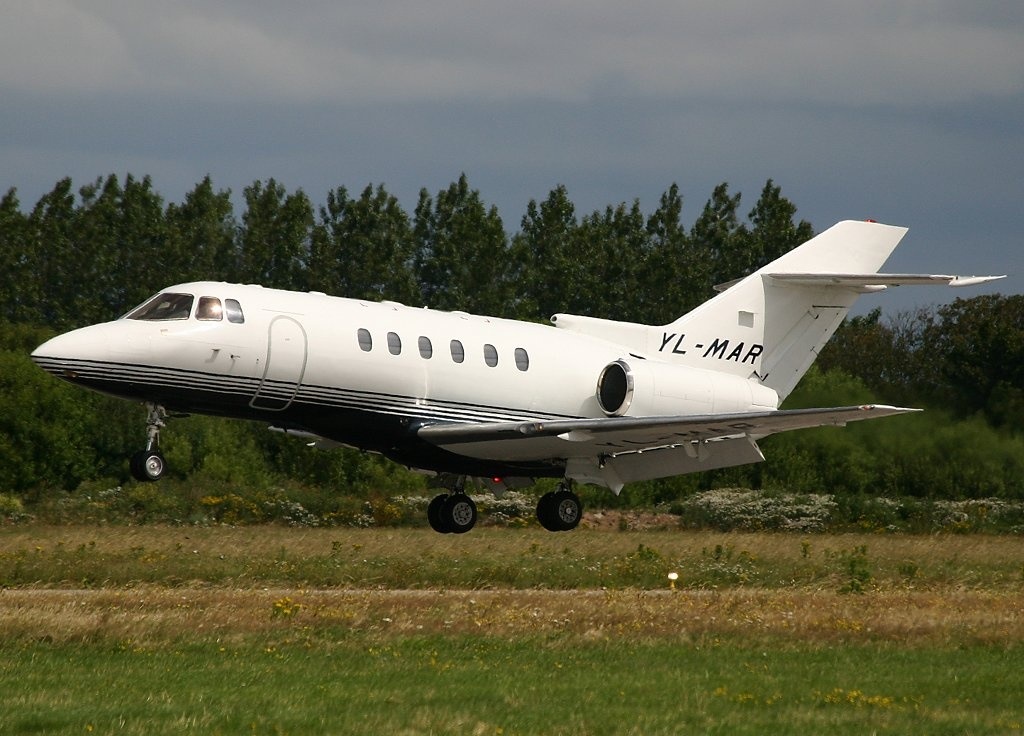
HS125 (Hawker 800) Business Jet)

The data for the HS125 Business jet are given in the table below. The aerodynamic model gives the lift, drag, and pitching moment coefficients as:

\begin{aligned} C_L &= C_{L_0} + C_{L_\alpha}\,\alpha + C_{L_{\delta_e}}\,\delta_e\\ C_D &= C_{D_0} + C_{D_\alpha}\,\alpha + C_{D_{\alpha^2}}\,\alpha^2\\ C_M &= C_{M_0} + C_{M_\alpha}\,\alpha + C_{M_{\delta_e}}\,\delta_e + C_{M_q}\,\hat{q}\\ \hat{q}&\triangleq \frac{Q\,\bar{c}}{V_f}\end{aligned}

Parameter	Symbol	Value
Mass	$m$	7500kg
Wing Area	$S$	32.8 $\text{m}^2$
Pitching Moment of Inertia	$I_{yy}$	84,309 $\text{kg m}^2$
MAC	$\bar{c}$	2.29m
Thrustline vertical displacement	$\Delta_{zT}$	-0.378m
Lift Coefficients	$C_{L_0},\, C_{L_\alpha},\, C_{L_{\delta_e}}$	0.895, 5.01, 0.722
Drag Coefficients	$C_{D_0},\, C_{D_\alpha},\, C_{D_{\alpha^2}}$	0.177, 0.232, 1.393
PM Coefficients	$C_{M_0},\, C_{M_\alpha},\, C_{M_{\alpha^2},\, C_{M_q}}$	-0.046, -1.087, -1.88, -7.055

The reduced nonlinear equations of motion can be constructed into a function eqnofmotion800:

To determine the transient aircraft response, first the trim state must be determined.

Trim State Determination

By definition, the trim case is found by setting the accelerations and angular velocities to zero. Hence the equations of motion become:

\begin{aligned} 0 &= T - D\cos\alpha + L\cos\alpha - mg\,\sin\Theta\\ 0 &= -L\cos\alpha - D\sin\alpha+ mg\,\cos\Theta\\ 0 &= M_A - T\Delta_{zT}\end{aligned}

The knowns in the above are flightspeed, $V_f$ , density (from altitude), $\rho$ , and climb angle/flight path angle $\gamma$ (setting $U_E$ and $W_E$ ). These may be solved via any means you like to get the reference trim state. An example of a Newton-Raphson solver¹ is included below as TrimState which finds trim using TotalForces:

For a trim input of sea-level and 120kn, the trim is found to be - $T = 13.84$ kN, $\delta_e = -0.98^\circ$ , $\Theta = 0.84^\circ$ . A quick sense check shows that the aircraft is slightly nose up (less than a degree) so the aerodynamic pitching moment from the wing/fuselage will be nose-up, and the elevator is deflected trailing edge up to balance the pitching moment.

Transient Simulation

For level flight (trim), the initial conditions are given from from the previous step - if the aircraft remains undisturbed, then there will be no variation in any of the parameters. The nonlinear equations cannot be solved analytically, so if the aircraft response to control inputs is desired, then a numerical scheme must be used.

The case of a positive elevator deflection corresponding to a stick-forward displacement will be explored. First, the response to a $\delta_e^\prime=1^\circ$ will be explored - this is equivalent to the pilot pushing the stick forward and holding it, keeping other controls constant.

The equations are solved numerically using scipy’s odeint (which is very similar to ODE45 in MATLAB)

Interactive demo

It should be noted that the values above are total values and NOT perturbational values. We can compare a linear model of the HS125 with the reduced nonlinear model, above - but rather than sourcing HS 125 data of unknown legacy, it makes more sense (but more work) to use the HS125 model to produce numerical derivatives based upon small perturbation theory using the model itself.

Numerical Linearisation of the Equations of Motion

This section shall stick with the HS 125 business jet. For the longitudinal equations of motion:

\begin{aligned} \begin{bmatrix} \dot{u}\\\dot{w}\\\dot{q}\\\dot{\theta}\end{bmatrix} &= \begin{bmatrix} X_u & X_w & 0 & -g\cdot\cos\theta_0\\ Z_u & Z_w & U_0 & -g\cdot\sin\theta_0\\ M_u^* & M_w^* & M_q^* & M_\theta^*\\ 0 & 0 & 1 & 0 \end{bmatrix}\begin{bmatrix} {u}\\{w}\\{q}\\{\theta^\prime} \end{bmatrix} + \begin{bmatrix} 0\\Z_{\delta_0}\\M_{\delta_0}^*\\0 \end{bmatrix}\left[\delta_0\right]\\ \dot{\vec{x}} &= \hspace{2cm} A\vec{x} + B\vec{u} \end{aligned}

\begin{aligned} M_u^*&\triangleq M_u + M_{\dot{w}}Z_u\,\,\,\,\,\,\,\,M_w^*\triangleq M_w+M_{\dot{w}}Z_w\,\,\,\,\,\,\,\,M_q^*\triangleq M_q+M_{\dot{w}}U_0\nonumber\\ M_{\delta_0}^*&\triangleq M_{\delta_0}+M_{\dot{w}}Z_{\delta_0}\,\,\,\,\,\,\,\,M_{\theta}^*\triangleq-M_{\dot{w}}g\sin\theta_0 \nonumber \end{aligned}

For each of the derivatives contained above, a central-difference approach may be utilised. That is, if the longitudinal force is a function of the aircraft states:

X = f\left(U, W, Q,\Theta_0,\delta_{e_0}\right)

then each of the stability derivatives may be expressed as a numerical partial derivative. For example

X_u = \frac{1}{m}\left.\frac{\partial X}{\partial u}\right|_0=\frac{1}{m}\left[\frac{f\left(U_0+\delta U,W_0,Q_0,\theta_0,\delta_{e_0}\right)-f\left(U_0- \delta U,W_0,Q_0,\theta_0,\delta_{e_0}\right)}{2\delta U}\right]

Note that the variable that the derivative is with respect to is altered, and the others are held constant - this is a partial derivative. This can be repeated for the remaining derivatives. This procedure has been used below to create stability derivatives.

ForcesandMoments gives values of the $X$ , $Z$ , and $M$ force and moments, and then NumerialDerivatives uses a central difference approach with ForcesandMoments to create the s

You will not be tested on things like this in an examination in this course, but it’s really in your interest to ensure that you can a) understand how this solver works and b) be confident you could write something that does the same job yourself. ↩

Comparison of the Linear and Nonlinear Equations of Motion: Aircraft Simulation

HS125 (Hawker 800) Business Jet)

Trim State Determination

Transient Simulation

Numerical Linearisation of the Equations of Motion

Footnotes