Aircraft Performancedraft

Questions and Solutions

The following comprises the theory that I expect you to have absorbed and be fluent in over the preceding module. Some questions have wordy answers whilst others have numerical answers. The numerical answers are provided, and the method is hidden in dropdowns in some cases, and completely hidden in the source ipynb notebooks in other cases.

A lot of the theory questions ask you to derive something. I do not include solutions to these questions - they are all ‘bookwork’ which is included in the notes. If you’re not able to answer them, ask on Slack.

Remember that you are expected to be writing your own code snippets rather than simply using this website as a calculator. I might be a real bastard and turn off the live code functionality during certain exams to enforce that.

Background Questions

These are not directly taught in this course, per se, but will prove your abilities to analyse aircraft data in order to even start the problems in Module 1. The following will test your understanding of the drag polar.

WT Data

A test is carried out on a 1:20 scale model of an aircraft in an atmospheric wind tunnel (ie $\rho = \rho_{SL}$ in the working section) at a speed of 20m/s. The model has a rectangular wing with a span of 1.70m and a chord of 0.24m.

$\alpha/^\circ$	-6	-3	0	3	6	9	12	15	18
$L\,\text{N}^{-1}$	-25	0	25	50	75	100	125	135	115
$D\,\text{N}^{-1}$	1.9	1.6	1.9	2.8	4.3	6.4	9.1	13.8	19.2

Perform the following data analysis and presentation:

Evaluate $C_L$ and $C_D$ for each incidence.
Plot $C_D$ against $C_L$ .
Plot lift/drag ratio $C_L$ / $C_D$ against $C_L$
Plot $C_D$ against $C_L^2$ .

and using these graphs, estimate:

The lift curve slope $a$ .
The zero-lift incidence $\alpha_{0L}$ .
The lift coefficient at zero lift, $C_{L0}$
The induced drag factors $K$ and $k$ .
The zero lift drag $C_{D0}$ (you can assume camber is negligible)
The maximum lift/drag ratio.
The approximate stall angle $\alpha_s$ .
The maximum lift $C_{Lmax}$

Answers

a= 4.78/rad

\alpha_{0L}= -3^\circ

C_{D0} = 0.016, K = 0.048, k=1.07

L/D_{max}\simeq 18

\alpha_S\simeq 15^\circ

C_{Lmax}\simeq 1.35

Conversion to flight data

The wind tunnel model described above is of an aircraft which weighs 300kN at full scale. It flies at maximum L/D at a height for which $\sigma$ = 0.25.

Determine the following:

The aircraft angle of attack
The airspeed, $V$ , and the required power at this condition
The minimum flight speed at this altitude
If the aircraft can produce 100kN thrust at sea level, what is the maximum speed at the altitude in the question
Comment on the answer to (4), and whether it is a realistic value.

The solutions are included below - note there is a choice to make in the equations regarding drag polar, which relate to the sparsity of the data. The $C_{L,md}$ can be taken from the raw data or from the drag model. Looking at the drag polar above, and the lift-to-drag ratio, to which both have been added, I think you can reasonably use the drag model but either value is acceptable.

Level Flight

Understanding the drag model

The basic non-dimensional drag equation for an aircraft at low speed is:

\begin{align*} C_D &= C_{D0} + K\cdot C_L^2\\ &= C_{D0} + \frac{k}{\pi\cdot AR}C_L^2 \end{align*}

Describe the significant of each term in the equation.

Answers

$C_D$ - Total drag coefficient $C_D\triangleq\frac{D}{\tfrac{1}{2}\cdot\rho\cdot V^2\cdot S}$

$C_L$ - Lift coefficient $C_L\triangleq\frac{D}{\tfrac{1}{2}\cdot\rho\cdot V^2\cdot S}$

$C_{D0}$ - Zero-lift drag - combination of skin friction and the part of form drag that does not vary with incidence.

$K$ - Induced drag effect $K\triangleq\frac{k}{\pi AR}$

$AR$ - Aspect ratio $AR\triangleq\frac{B^2}{S}$

$k$ - Induced drag factor - if wing has a non-elliptical lift distribution ( $k>1$ )

Understanding EAS

Explain the concept of Equivalent Air Speed (EAS). Writing the drag equation in dimensional form, demonstrate that using EAS enables us to plot a single curve of drag vs. speed for all altitudes. Include in your answer a sketch of the variation of drag with speed.

So what is EAS...?

Consider an aircraft flying at True Air Speed (TAS or $V$ ) at some altitude $h$ where the air density is given by $\rho$ . The Equivalent Air Speed (EAS or $V_E$ ) is the speed at which, if flown at ISA sea-level density ( $\rho_{SL}=1.225\frac{\text{kg}}{\text{m}^3}$ ), would give the same dimensional aerodynamic loads for the same aerodynamic configuration \ie constant $C_L$ etc.

\begin{equation*} V_E\triangleq V\sqrt\frac{\rho}{\rho_{SL}}=V\sqrt{\sigma} \end{equation*}

Taking the drag equation from question (a), and dimensionalising, we get:

\begin{align*} D &= C_{D0}\cdot\frac{1}{2}\cdot\rho\cdot S\cdot V^2 + K\cdot C_L\cdot\frac{1}{2}\cdot\rho\cdot V^2\cdot S \end{align*}

i.e.,

\begin{align*} D &= f(V,\rho)\\ &= f(V, h) \end{align*}

So if we plot dimensional drag vs true airspeed, the curves will be different for each altitude. If we take the definition for $V_E$ , rearrange for $V$ , we may substitute into the dimensional drag equation and get:

\begin{align*} D &= C_{D0}\cdot\frac{1}{2}\cdot\rho_{SL}\cdot S\cdot V_E^2 + K\cdot C_L\cdot\frac{1}{2}\cdot\rho_{SL}\cdot V_E^2\cdot S \end{align*}

since $\rho_{SL}$ is constant with altitude,

\begin{align*} D &= f(V_E) \end{align*}

Hence drag as a function of EAS is constant with altitude. QED. We can sketch the variation of drag with EAS:

dragbreakdown

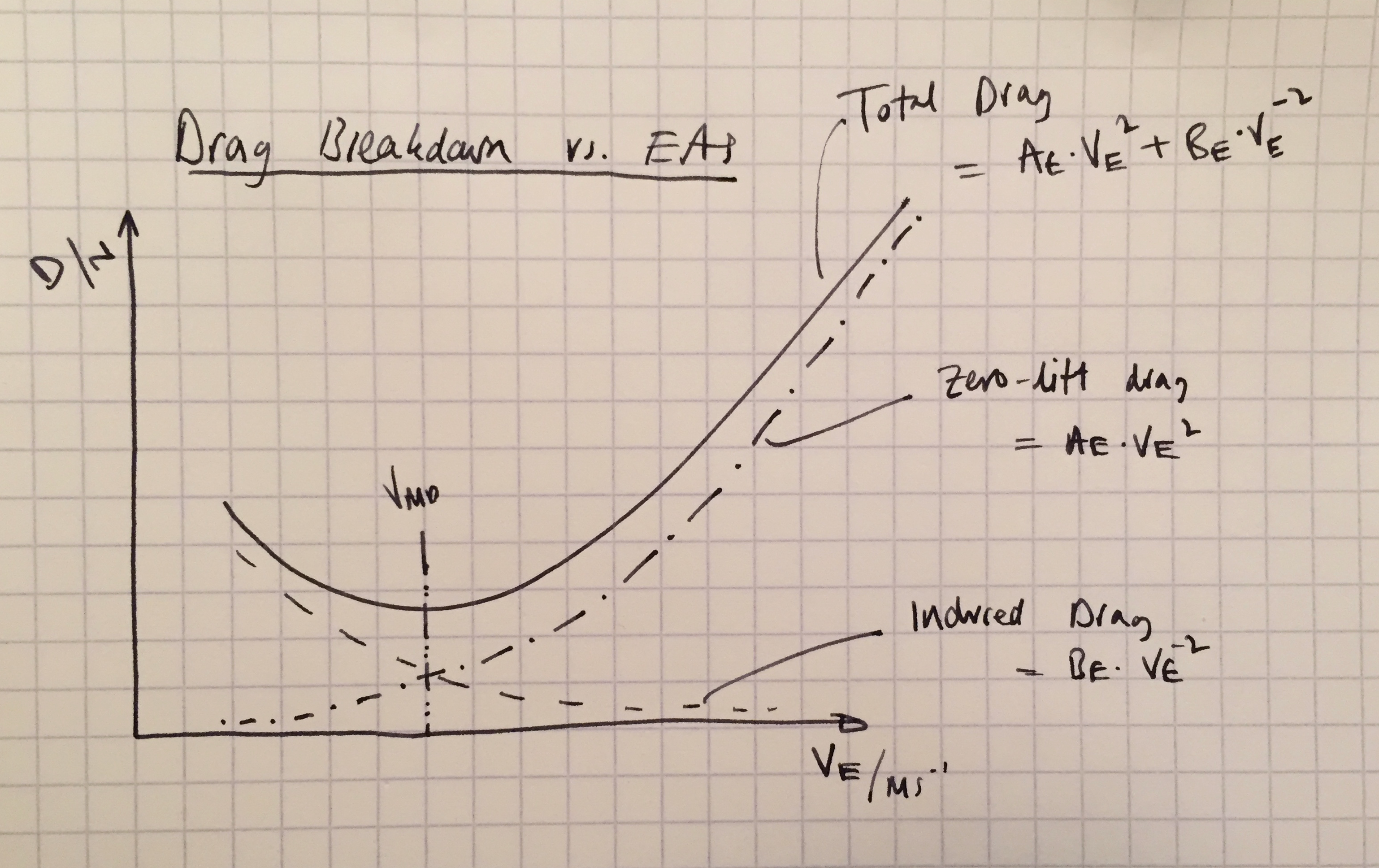
where:

\begin{align*} A_E &= C_{D0}\cdot\frac{1}{2}\cdot\rho_{SL}\cdot S\\ B_E &= \frac{K\cdot W^2}{\frac{1}{2}\cdot\rho_E\cdot S} \end{align*}

Understanding power required

Determine the lift coefficient and drag coefficient when flying at minimum \textsl{power}, and hence show that the corresponding true airspeed is:

\begin{equation*} V_{mp} = \left[\frac{2W}{\rho S}\right]^{\tfrac{1}{2}}\left[\frac{K}{3\cdot C_{D0}}\right]^{\tfrac{1}{4}} \end{equation*}

Bookwork derivation

From the question above we have:

\begin{align*} D &= A\cdot V^2 + B\cdot V^{-2} \end{align*}

where

\begin{align*} A &= C_{D0}\cdot\frac{1}{2}\cdot\rho\cdot S\\ B &= \frac{K\cdot W^2}{\frac{1}{2}\cdot\rho\cdot S} \end{align*}

power (P) is the rate of work done, or the thrust multiplied by velocity:

\begin{align*} P &= T\cdot V\ \end{align*}

for steady cruise, $T=D$

\begin{align*} P &= D\cdot V\\ &= A\cdot V^3 + B\cdot V^{-1} \end{align*}

minimum power at $\frac{\text{d}P}{\text{d}V}=0$

\begin{align*} \frac{\text{d}P}{\text{d}V} &= 3A\cdot V^{1} - B\cdot V^{-3}=0\\ \implies 3AV_{mp}^4 &= B\\ V_{mp}^4 &= \frac{B}{3A}\\ V_{mp} &= \left[\frac{B}{3A}\right]^{\tfrac{1}{4}}\\ &= \left[\frac{K\cdot W^2}{\frac{1}{2}\cdot\rho\cdot S}\cdot\frac{2}{3\cdot\rho\cdot C_{D0}\cdot S}\right]^{\tfrac{1}{4}}\\ &= \left[\left\{\frac{2\cdot W}{\rho\cdot S}\right\}^2\cdot\frac{K}{3\cdot C_{D0}}\right]^{\tfrac{1}{4}}\\ &= \left[\frac{2W}{\rho S}\right]^{\tfrac{1}{2}}\left[\frac{K}{3\cdot C_{D0}}\right]^{\tfrac{1}{4}}\hspace{1cm}\text{QED} \end{align*}

Numerical Drag Equation Manipulation

A jet trainer has the drag equation:

\begin{equation*} C_D = 0.018 + 0.016\cdot C_L^2 \end{equation*}

and a minimum power speed of 60m/s EAS. What is the thrust to weight ratio required to cruise at 200m/s EAS?

Please attempt the solution yourself first, or you'll learn nothing...

Knowns:

\begin{align*} C_{D0} &= 0.018\\ K &= 0.016\\ V_{Emp} &= 60\text{m/s}\\ V_{E} &= 60\text{m/s} \end{align*}

Required:

\begin{align*} \frac{T}{W}_{200EAS} &\therefore \frac{D}{W}_{200EAS} \end{align*}

There are a few ways to go about this equation, you can get $C_{Lmp}$ by differentiating the power equation for $C_L$ , and determine $C_D/C_L$ which is the same as $T/W$ . Alternatively, you can do the following, which is how I would solve it:

First rearrange the minimum power speed from the previous question for the unknowns ( $W$ and $S$ ):

\begin{equation*} \frac{W}{S} = \left(V_{mp}\cdot\left[\frac{K}{3\cdot C_{D0}}\right]^{-\tfrac{1}{4}} \right)^2\cdot\frac{\rho}{2} \end{equation*}

we want $\frac{D}{W}$ so:

\begin{align*} \frac{D}{W} &= \frac{1}{W}\left\{A_E\cdot V^2 + B_E\cdot V^{-2}\right\}\\ &= C_{D0}\cdot\frac{1}{2}\cdot\rho_{SL}\cdot \left[\frac{W}{S}\right]^{-1}\cdot V_E^2 + \frac{K}{\frac{1}{2}\cdot\rho_{SL}}\cdot\frac{W}{S}\cdot V_E^2\cdot\\ &= C_{D0}\cdot\left\{V_{mp}\cdot\left[\frac{K}{3\cdot C_{D0}}\right]^{-\tfrac{1}{4}} \right\}^{-2}\cdot V_E^2 + K\cdot\left\{V_{mp}\cdot\left[\frac{K}{3\cdot C_{D0}}\right]^{-\tfrac{1}{4}} \right\}^2 \cdot V_E^{-2} \end{align*}

which, if we insert all the values above, yields $D/W=T/W=0.1115$

Minimum drag speed derivation

Working from first principles show that the the expression for the minimum drag speed of a conventional aircraft is given by:

\begin{equation*} V_{MD} = \left[\frac{2W}{\rho S}\right]^{\tfrac{1}{2}}\left[\frac{K}{C_{D0}}\right]^{\tfrac{1}{4}} \end{equation*}

where all the symbols have their usual meaning. You can assume a knowledge of the lift and drag coefficients’ meaning and definitions.

Bookwork derivation

We assume that the drag comprises a component that is lift-independent - $C_{D0}$ , due to the combination of form drag and skin friction drag, and a second part that rises linearly with the square of the lift due to induced drag, and the $\alpha$ -variation of the form drag - $K\cdot C_L^2$ . \ie

begin{align*} C_D &= C_{D0} + K\cdot C_L^2 \end{align*}

dimensionalising by multiplying by $q_\infty\cdot S$ :

\begin{align*} \implies D &= C_{D0}\cdot\frac{1}{2}\rho\cdot S\cdot V^2 + K\cdot C_L^2\cdot\frac{1}{2}\cdot S\cdot V^{-2}\\ &= A\cdot V^{2} + B\cdot V^{-2}\\ \end{align*}

with $A=C_{D0}\cdot\frac{1}{2}\cdot\rho\cdot S$ and $B=\frac{KW^2}{\frac{1}{2}\cdot\rho\cdot S}$ . To find the variation of drag with lift, we can differentiate the above expression wrt V, and find the zero point:

\begin{align*} \frac{\text{d}D}{\text{d}V} &= 2\cdot A\cdot V^{-1} - 2\cdot B\cdot V^{-3}\\ \implies V_{mp} &= \left[\frac{B}{A}\right]^{\tfrac{1}{4}}\\ &= \left[\frac{2W}{\rho S}\right]^{\tfrac{1}{2}}\left[\frac{K}{C_{D0}}\right]^{\tfrac{1}{4}}\text{ QED} \end{align*}

Numerical Minimum Drag Speed

An aircraft with a wing area of 20m $^2$ and drag given by $C_{D0}=0.015$ and $K=0.04$ is flying at an altitude of 6km, at its minimum drag speed.

If the engine thrust is 2500N, what is the speed and weight of the aircraft?

The thrust is now increased by 10%, find:

The new steady flight speed if the aircraft is held level at the same altitude.
If the lift curve slope is 5.7/rad, what change in aerodynamic incidence is required to maintain level flight at these new speeds
The steady rate of climb, and the climb angle achieved if the aircraft’s speed is unchanged.

The hidden sections below correspond to solution, and answer for parts 1 through 3.